Using mcrl2-gui
All tools in the mCRL2 toolset are, besides their command-line interface, also available through the graphical user interface in mcrl2-gui. In this section we show by example how to use the toolset through the graphical user interface.
Start the mcrl2-gui tool by either typing mcrl2-gui on the command line,
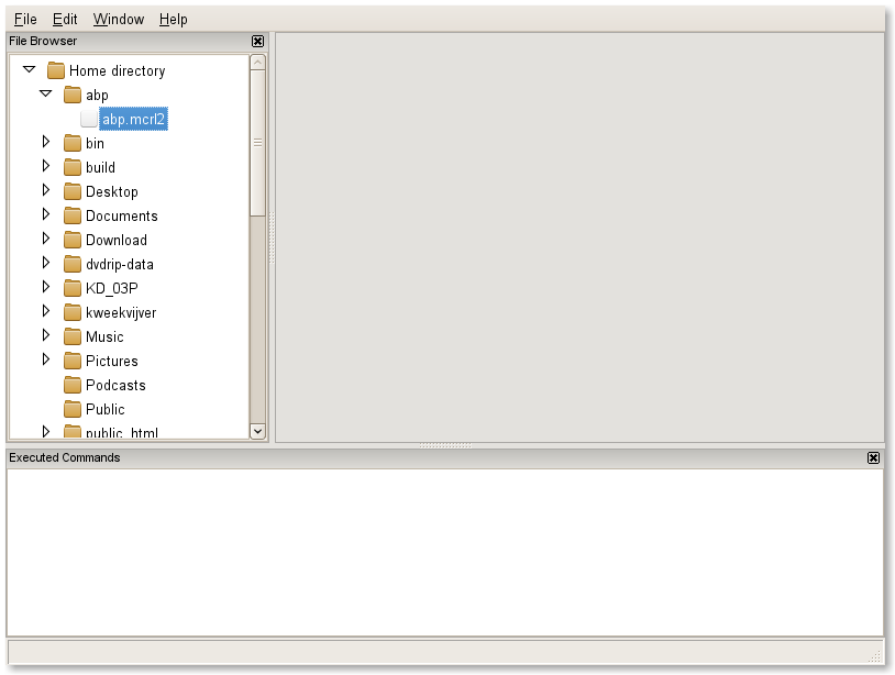
or double click onto the mcrl2-gui icon. The mcrl2-gui window appears,
showing two panels. One panel displays in a tree-view structure the files on
disk, called “File Browser”, right-clicking a file in this panel will show the
supported operations (Transformation, Report, etc.) for the selected file. The
other panel displays the commands that have been executed throughout the
transformation and analysis, called “Executed commands”. Throughout the
tutorial, another panel will appear to configure and run tools. This panel is
called the “Configuration panel”.
In this tutorial the analysis and transformations are performed on the
alternating bit protocol. The corresponding mCRL2 specification can be
downloaded (abp.mcrl2).
or be found in the examples/academic/abp/ directory of your mCRL2
installation.
|
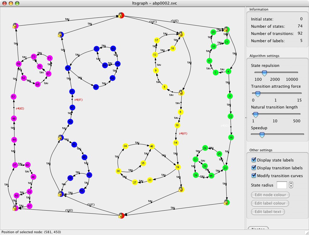
The ltsgraph tool, showing the statespace of the alternating bit protocol. |
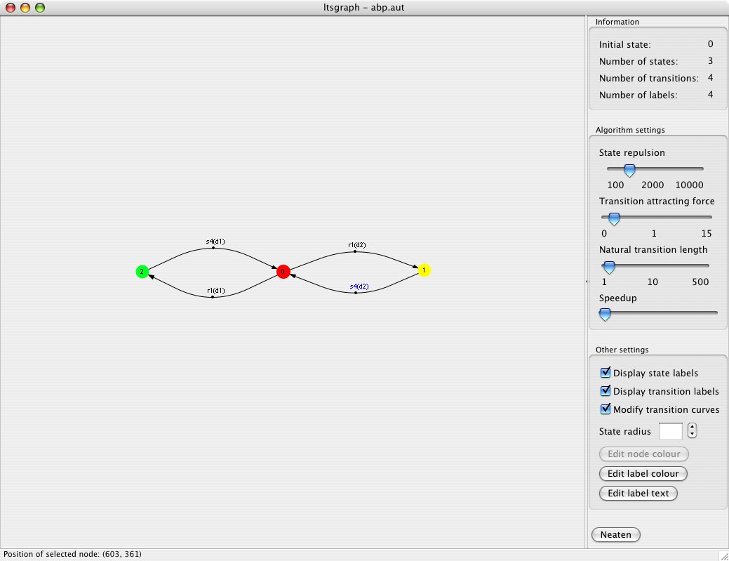
The ABP statespace after branching bisimulation reduction. |
|
Obtaining a linear process specification
Navigate with help of the file browser to the mcrl2 specification, that contains
a behavioural description of the alternating bit protocol, named abp.mcrl2.
After right-clicking on the file abp.mcrl2, a pop up menu shows up that
displays the available operations that can be applied to the selected file.
Operations differ per file, per extension and per folder. To transform the mcrl2
specification into a linear specification, we need to use the tool
mcrl22lps. This tool can be found under
. After selecting mcrl22lps, the
mcrl2-gui displays the configuration panel, as shown below.
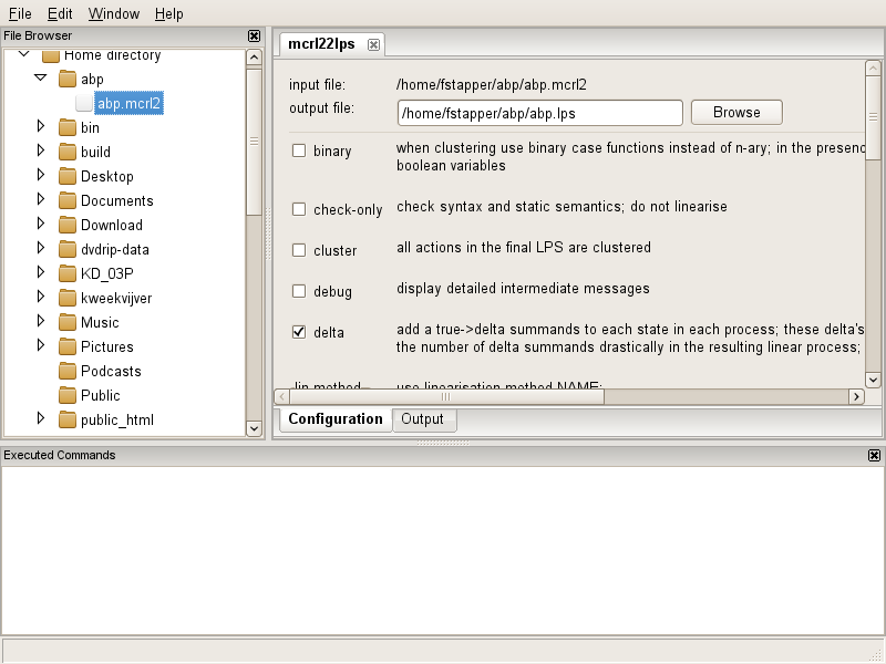
The configuration panel displays the input file, a suggestion for a possible output-file, the different linearisation options that can be applied and a “run” button to execute the transformation. The “run” button can be found by scrolling down the panel. We choose to alter the suggested file name to “abp.lps” and press the run button. After the button has been pressed, mcrl22lps generates the output file. Notice that the file browser automatically selects the file, after it has been successfully created.
Generating a labelled transition system
Now we right-click on the new created file. Note that files with an .lps
extension, have more tools that can use the input for the analysis or
transformation. To generate a labeled transition system, we apply the
transformation lps2lts (). By selecting lps2lts, a new tab with options pops up in the
configuration panel. For the moment we ignore all options, and simply click the
run button. A new file called abp.lps2lts00.lts is generated.
ltsgraph and ltsconvert
There are several tools that work on .lts files. In particular, they can be
visualized using the tool ltsgraph. When starting ltsgraph
(), the states and transitions occur at
random places. The states and labels can be moved around using the left mouse
button. By pushing the neaten button, a simple positioning algorithm will start
to optimize the picture. States can still be dragged around while the diagram is
being optimized. Using the right mouse button (Ctrl+mouse on Mac OS X) states
can be locked, which prevents them from being moved around automatically. The
resulting layout can be saved and exported to scalable graphics format (SVG) or
LaTeX (pstricks). It is also possible to colour individual states and to change
the curvature of transitions.
Another tool that works on labelled transition systems, is ltsconvert.
This is a very versatile tool to translate various
representations of labelled transitions systems to each other (e.g. the
.aut, .lts and .fsm formats). Moreover, it can apply strong,
branching and trace equivalence reductions on the transition systems. Let’s
apply ltsconvert to abp.lps2lts00.lts. Set the branching bisimulation
reduction option, and generate the reduced transition system (abp.aut). Note
that ltsconvert generates a file that conforms to a .aut specification,
given the file extension. Visualizing it, by using ltsgraph, yields the third
picture above: a transition system with three states. For those who know the
alternating bit protocol, this exactly depicts its desired external behaviour,
in case it has two data items d1 and d2.
ltsview and diagraphica
Using ltsconvert it is also possible to create a .fsm file, which is the
input format for two other graphical tools, namely ltsview and
diagraphica. Start ltsconvert on abp.lts. Select as
an output file abp.fsm and put abp.lps as the linear process
specification to be used. This last step is needed because the .fsm format
requires the names, sorts and values of the process variables in each state.
Without it, both diagraphica and ltsview cannot show the values of the
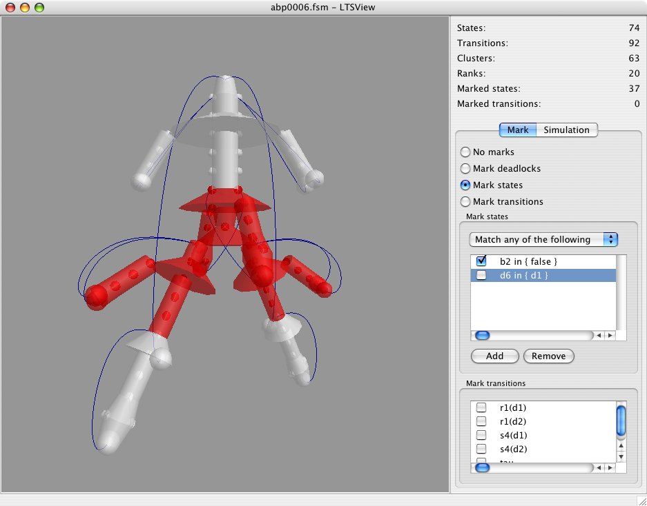
variables in each state, strongly crippling their functionality. The state space
that shows up in ltsview can be navigated using the mouse. It can be coloured
on the basis of the variables in each state, but also using transitions or the
existence of deadlock. Note that for the alternating bit protocol it is possible
to show the individual states, transitions and backpointers. For larger state
spaces (with hundreds of thousands of states), showing too much detail slows the
tool down dramatically.
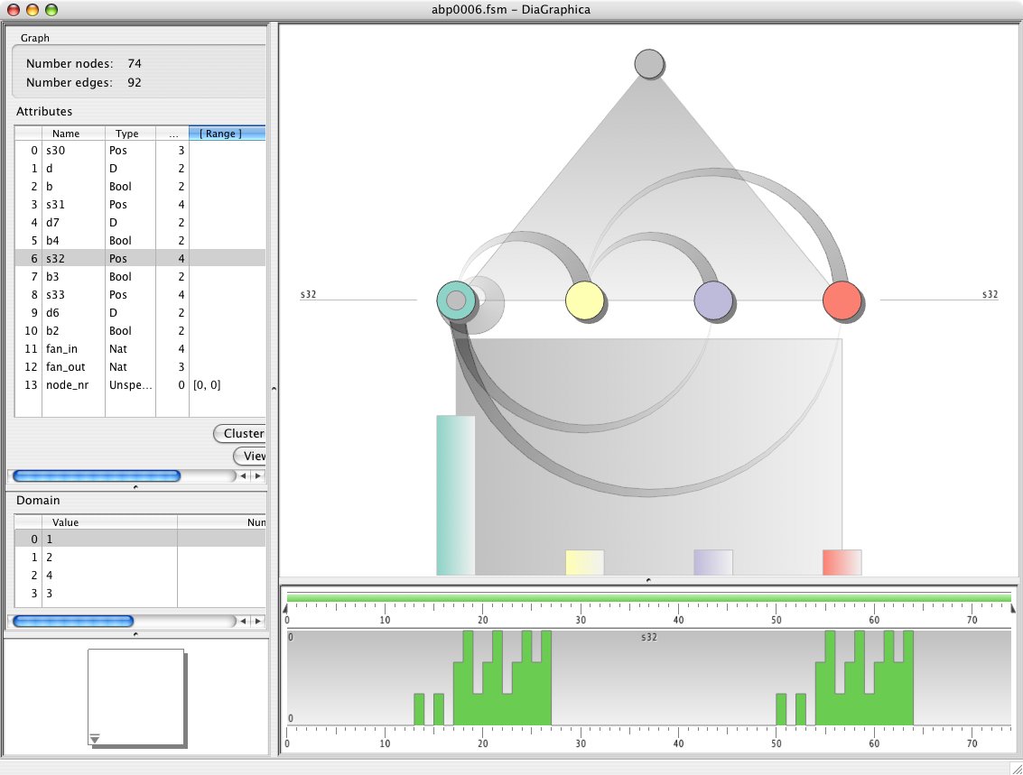
Diagraphica visualises process parameters. |
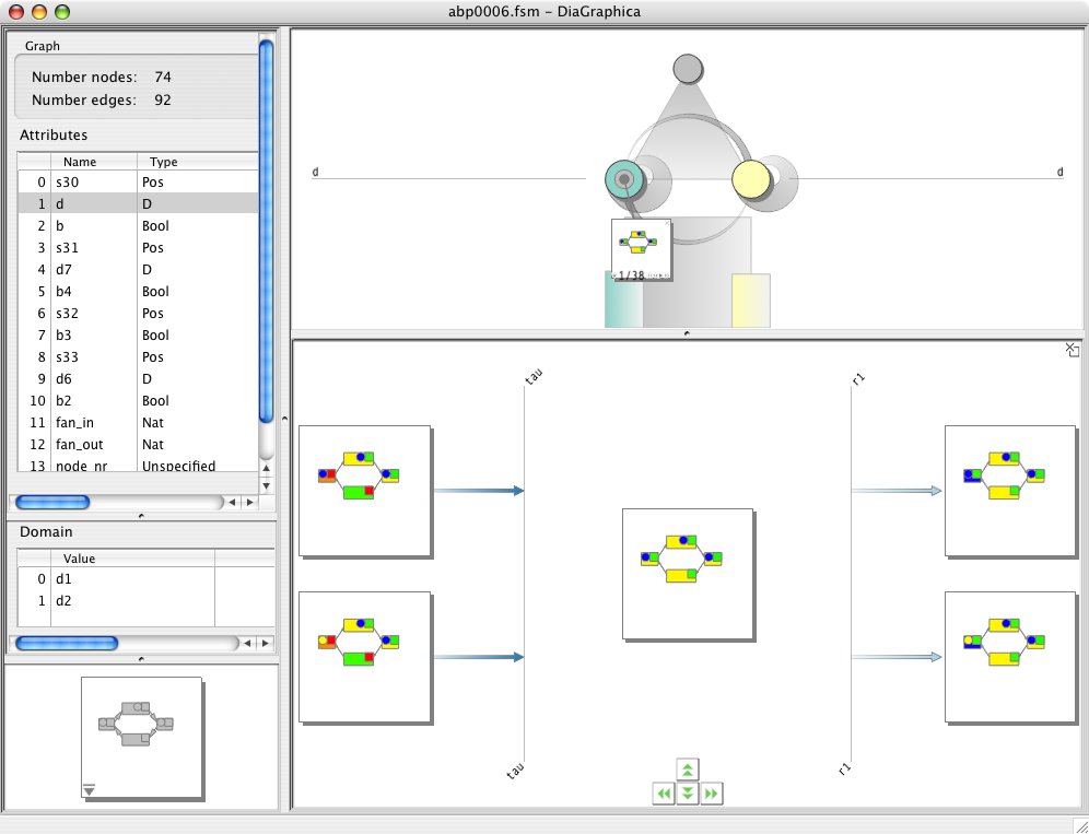
Diagraphica as a graphical simulator. |
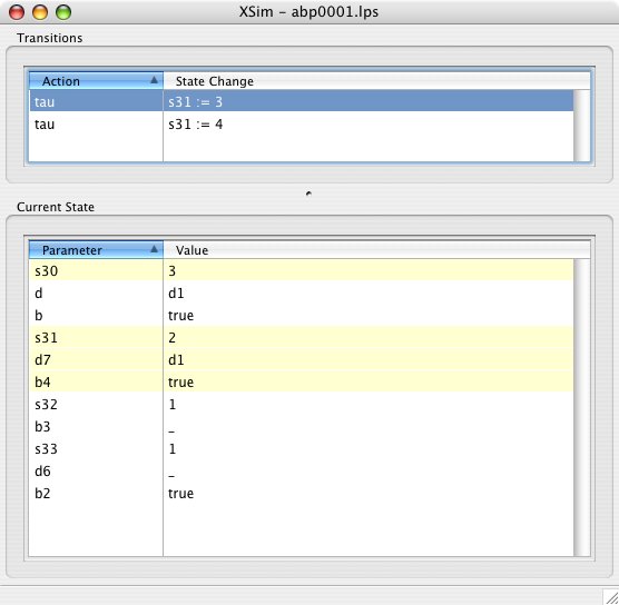
The lpsxsim tool simulating the alternating bit protocol. |
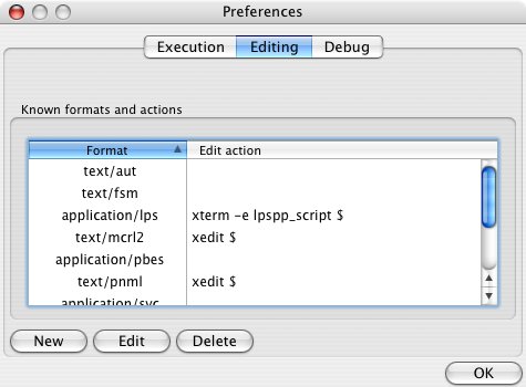
The edit window allows to use external editors. |
The tool diagraphica allows to visualize the process parameters that make up each state. If diagraphica is started, the process parameters are listed in the window to the left. For the alternating bit protocol these are s30, d, b, s31, etc. Using the mouse a subset of these variables can be selected and the whole state space is projected onto the selected variables by pushing the Cluster nodes button. Using different options under in the main menu, it is possible to visualize properties of the selected variables.
In the view on the right, the circles represent aggregated states. The circular shapes between these nodes are aggregated transitions, and must be read clockwise. It is possible to get an impression of the distribution of all values in the state space by switching to the trace view. By selecting some variables and performing a trace view, the values of the selected variables of all states are graphically represented in the window at the bottom. The result looks as in the leftmost picture above.
Another option of diagraphica is to graphically simulate the process. A
graphical view of the process can be edited in edit mode. The file
abp.dgd, which can be downloaded (abp.dgd),
contains an initial layout, but in edit mode any layout can be made. Using the
edit DOF option, that shows up when clicking an object in edit mode,
a pop up window appears showing which colours, shape, position and even
transparency of objects can be made dependent on the state of the process. Back
in analysis mode, with the simulation view, it is possible to observe how the
layout changes while doing simulation steps.
Simulating a linear process specification
The tool lpsxsim operates on .lps files and can be used to
simulate a process. The third picture above shows its interface. A very useful
feature of lpsxsim is its capability to load traces. Traces generated with
other tools (such as lps2lts) can easily be investigated in this way. For this
purpose there are a trace view possibility and capabilities to walk back and
forth through the trace. The tool lpsxsim can be interfaced to external viewers
to build realistic prototype simulation of the modelled artefacts.
Setting an external editor in mcrl2-gui
mcrl2-gui uses the system defined editors that belong to a particular file
extension. If a user wants (or needs) to define/override an editor, this can be
accomplished in the preferences window (). For each file extension an associated editor can be set. Use the
%s symbol to indicate the current file on which the editor must operate.
Concluding remarks
With these tools many basic analyses on behavioural descriptions can be performed. All available tools are described in the Tool documentation, although generally in terms of command line invocation.