Process syntax
Process expressions
Action ActIdSet MultActId MultActIdList MultActIdSet RenExpr RenExprList RenExprSet CommExpr CommExprList CommExprSet DataExprUnit ProcExpr
Action ::=Id('('DataExprList')')? ActIdSet ::= '{'IdList'}' MultActId ::=Id('|'Id)* MultActIdList ::=MultActId(','MultActId)* MultActIdSet ::= '{'MultActIdList? '}' RenExpr ::=Id'->'IdRenExprList ::=RenExpr(','RenExpr)* RenExprSet ::= '{'RenExprList? '}' CommExpr ::=Id'|'MultActId'->'IdCommExprList ::=CommExpr(','CommExpr)* CommExprSet ::= '{'CommExprList? '}' DataExprUnit ::=Id|Number| 'true' | 'false' | '('DataExpr')' |DataExprUnit'('DataExprList')' | '!'DataExprUnit| '-'DataExprUnit| '#'DataExprUnitProcExpr ::=Action|Id'('AssignmentList? ')' | 'delta' | 'tau' | 'block' '('ActIdSet','ProcExpr')' | 'allow' '('MultActIdSet','ProcExpr')' | 'hide' '('ActIdSet','ProcExpr')' | 'rename' '('RenExprSet','ProcExpr')' | 'comm' '('CommExprSet','ProcExpr')' | '('ProcExpr')' |ProcExpr'+'ProcExpr| 'sum'VarsDeclList'.'ProcExpr|ProcExpr'||'ProcExpr|ProcExpr'||_'ProcExpr|DataExprUnit'->'ProcExpr|DataExprUnit'->'ProcExpr'<>'ProcExpr|ProcExpr'<<'ProcExpr|ProcExpr'.'ProcExpr|ProcExpr'@'DataExprUnit|ProcExpr'|'ProcExpr| 'dist'VarsDeclList'['DataExpr']' '.'ProcExpr
The non-terminal ProcExprNoif is equal to ProcExpr, except
that no if-then or if-then-else productions are allowed. It recurses back
into ProcExpr where this non-terminal is enclosed by brackets;
otherwise, it stays in ProcExprNoIf.
Process equation
ProcDecl ProcSpec
ProcDecl ::=Id('('VarsDeclList')')? '='ProcExpr';' ProcSpec ::= 'proc'ProcDecl+
Process specifications
Processes are the most important entities in a process specification. They are used to describe the behaviour of some system or component. The most basic process is the sequential process which can carry data parameters. This data can influence the behaviour of the process via the conditional and summation constructs. Processes can be combined using the parallel composition operator to obtain more complex processes. Operators exists for enforcing synchronous communication between parallel processes. Also, some actions that a process performs can be renamed or hidden. The latter operation is useful to separate internal behaviour from externally visible behaviour. Finally, time can be added to processes.
Actions
The primitive operation of processes is the action. An action represents an event of any kind, be it sending a message, printing a letter on a screen or shaking hands. Such events are declared by:
act send: Message;
    print: Letter # Screen;
    Shake_hand;
where Message, Letter and Screen are the sorts of the objects that
are exchanged in such an event. An action can have 0 or more of such arguments,
separated by # symbols.
Process algebra
Actions can be combined to describe behaviour, which represents all possible
sequences of actions that can be done. The main operators are sequential
composition, the dot ., which puts two behaviours in sequence, and the
alternative composition, the plus +, which represents the choice between two
behaviours. So, in the following P is the process where actions a, b and c can
happen in sequence. In the process Q there is a choice between actions d and e.
Finally, the process R consists of first doing a choice between a and b,
followed by a sequence of c, d and e.
act a, b, c, d, e;

proc P = a . b . c;
     Q = d + e;
     R = (a + b) . c . d . e;
Whether a process P + Q behaves as P or as Q is determined by the
first action that either P or Q carries out.
By using process variables at the right-hand side, recursive behaviour can be specified. A process that iteratively performs a read and a write action is written as:
act read, write;
proc P = read . write . P;
init P;
The keyword init indicates that the process starts with the process P.
Actions are allowed to occur simultaneously. In this case we speak about
multi-actions. A multi-action is a sequence of actions that are separated by
bars. E.g. a|b|...|z. If we reconsider the example above, but we want to
express that reading and writing must happen at the same time, this can be
specified by:
act read, write;
proc P = (read | write) . P;
init P;
Multi-actions are an effective weapon against the state space explosion problem. By grouping several actions into one multi-action, the number of states in a specification can be reduced.
The empty multi-action is the so-called hidden or internal action, which is
written as tau. The hidden action cannot be observed. It is not very useful
when specifying the behaviour of processes, but it is essential when it comes to
analysing processes.
There is one special process called deadlock, written as delta, which
denotes a process that cannot perform anything. In particular nothing can happen
after delta. So, the process delta . a and delta are the same.
Adding data
Processes can carry zero or more data parameters. For instance a clock that counts its ticks can be specified as follows:
act tick;
proc Clock(n: Nat) = tick . Clock(n + 1);
init Clock(0);
Also actions can have one or more arguments. So, we can extend the clock by showing the current time.
act tick;
    show: Nat;
proc Clock(n:Nat) = tick.Clock(n + 1)
                  + show(n) . Clock(n);
init Clock(0);
In practice, it often happens that processes carry a large number of parameters, while only a small number of these parameters need to be updated when the process is referenced. For this purpose, an assignment-like syntax is provided such that only the updated values need to be specified. Using these so-called process reference assignments, the above example becomes:
act tick;
    show: Nat;
proc Clock(n:Nat) = tick . Clock(n=n + 1)
                  + show(n) . Clock();
init Clock(0);
Conditions
We can let data influence the course of events by adding conditions to the
process. We write c -> p for “if c then do process p” and
c -> p <> q for “if c then do proces p else do process q”. For
instance, the clock above can be forced to count modulo 100, and it may only be
reset if n is smaller than 50.
act tick, reset;
proc Clock(n: Nat) = (n < 99) -> tick . Clock(n + 1)
                              <> tick . Clock(0)
                   + (n < 50) -> reset . Clock(0);
init Clock(0);
Summation
The sum operator allows to formulate the choice between a possibly infinite number of processes in a very concise way. In other formalisms, and in semi-formal texts, the sum operator is often written using the choice operator.
The process sum n: Nat . p(n) can be seen as a shorthand for p(0) + p(1) +
p(2) + .... The use of the sum operator is often to indicate that some value
must be read, i.e., the process wants to read either a 0 or a 1 or a 2, etc.
So, a buffer that reads some natural number and subsequently delivers it again
can be compactly specified by:
act read, write: Nat;
proc Buffer = sum n: Nat . read(n) . write(n) . Buffer;
init Buffer;
Looking at the example of the clock, the clock can be set to a particular time
using a sum operator and a set action:
act tick;
    set: Nat;
proc Clock(n: Nat) = tick . Clock(n + 1)
                   + sum m: Nat . set(m) . Clock(m);
init Clock(0);
If sum operators are used over infinite domains, such as Nat, then it is not
possible to simulate these, or generate a state space. This for instance holds
for the clock with the set action. In general, however, sums over infinite
domains are used to read data from other processes. This is proper, and even
encouraged, use of the mCRL2 toolset. All tools are optimised to deal with such
situations. In general no enumeration of data elements takes place in such a
situation.
There are situations where sums over infinite domains can be used safely for simulation or state space generation. For instance when there are conditions that restrict the domain. A typical example is the following:
act show: Nat;
proc P = sum n: Nat. (n < 10) -> show(n) . P;
init P;
Here the variable in the sum operator is restricted by a condition. Using the
constructors of the data domain Nat the tools will figure out that only the
finite set of numbers under 10 are relevant. This does not only work for natural
numbers, but for any constructor sort.
Note that when using the toolset symbolically (e.g. by symbolically solving modal formulas, proving invariants, or calculating confluence) there is no finiteness constraint at all on the sum operators.
Parallel composition
Processes can be put in parallel using the parallel operator. E.g. if p and
q are processes, the expression p || q represents the processes p
and q executing in parallel. More precisely, the actions of p and q
are executed in an interleaved fashion.
For example consider the process a || b (for actions a and b). This
process is equal to the following, where the a and b are not only
interleaved, as there is also a multi-action where a and b happen
simultaneously:
a . b + b . a + a | b
Note that parallel behaviour can easily become quite complex. For instance the
simple looking parallel process a . b || c . d is equal to the sequential
process:
  a . (b . c . d + b|c . d + c . (b . d + d . b + b|d))
+ c . (d . a . b + a|d . b + a . (b . d + d . b + b|d))
+ (a|c) . (b . d + d . b + b|d)
One of the major reasons why the analysis of behaviour is complex, lies in exactly this explosion of possibilities of parallel processes. It is virtually impossible to imagine all possible interleavings of actions.
The current implementation of the linearization procedure in mcrl22lps does not support recursive paralellism, e.g. processes like
proc X = a . (X || X)
cannot be handled. The same holds for the allow, block, hide and
comm operators that can not be used within recursive processes.
Communication and allow
We have seen in the previous section that parallel processes can have many interleavings, and some actions of parallel processes happen simultaneously. So, one process can do a send action and another reads, via a read action:
send || read = send . read + read . send + send|read
The intention is that send and read must happen at the same time (i.e. must
communicate) and can not happen as single isolated actions. In order to achieve
this there are two operators: comm and allow.
The comm({a|b -> c}, p) operator says which multi-actions are renamed to a
single action. It says that actions a and b must communicate to c in
process p. Concretely, in any multi-action of p all occurrences of
a|b are replaced by c, provided that the data that a and b
carry, match.
The allow({c}, p) operator says that besides the empty multi-action tau,
only multi-actions consisting of a single c are allowed in p. All other
actions are blocked. The allow operator can also permit multi-actions to happen,
as in allow({a|b, c|d}, p). In such a case the arguments of the allowed
multi-actions can differ.
The following expression enforces the desired communication in the example with read and write:
allow({c}, comm({send|read -> c}, send || read))
Transfering data can be done easily in this scheme. So, assume one process sends
a natural number n, which is read and processed by another process. This
could be specified by:
allow({c},
  comm({send|read -> c},
    send(n) . p || sum m: Nat . read(m) . q(m)
))
Here, q(m) is the process that uses the value m. The process above
actually behaves as
c(n) .
allow({c},
  comm({send|read -> c},
    p || q(n)
))
or in other words, the communication took place and the value n is neatly
handed over to q.
More components can be put in parallel. As a larger example we show how the four
components of the alternating bit protocol are assembled together. The process
S(true) is the sending protocol entity with initial bit true. The process
R(true) is the receiving entity, also with initial bit true. The
processes K and L model unreliable channels. The actions r1 and
s4 are external actions. Actions starting with a c are communications.
The action i represents an internal action in the channels that determine
whether data is lost or not.
init allow({r1,s4,c2,c3,c5,c6,i},
       comm({r2|s2->c2, r3|s3->c3, r5|s5->c5, r6|s6->c6},
         S(true) || K || L || R(true)
     ));
The complete description of the alternating bit protocol can be found in the file abp.mcrl2 in the directory examples/academic in the distribution of the toolset.
There is a dual operator of the allow operator. This is the encapsulation or
block operator that can block single actions. If a single action that is blocked
occurs in a multi-action the whole multi-action is renamed to delta. E.g. the
expression block({b}, a || b) is equal to a . delta.
Rename and hide
A convenient operator that is not used very often is the renaming operator,
which allows to rename action labels. E.g. rename({a -> b, c -> d}, p)
renames action a in p to b, and action c in p to d. The
operator is useful if certain processes must be used several times in a system,
and have different communication patterns each time.
It is possible to hide actions, which means that they are not visible anymore in
multi-actions. E.g. hide({a}, a|b) equals b, as a is hidden. Using
hiding it is possible to indicate that certain actions can no longer be observed
by the outside world. For instance with the alternating bit protocol, it might
be useful to indicate that the communications c2, c3, c5, c6 and the
internal choice i are not visible. This is done as follows:
init hide({c2,c3,c5,c6,i},
       allow({r1,s4,c2,c3,c5,c6,i},
         comm({r2|s2 -> c2, r3|s3 -> c3, r5|s5 -> c5, r6|s6 -> c6},
           S(true) || K || L || R(true)
     )));
It is important to use hide, allow and comm in this way. Changing
the order of these operators will lead to partial hiding of multi-actions, which
causes the number of summands in the linear process to grow. This makes analysis
and simulation of the process behaviour much harder.
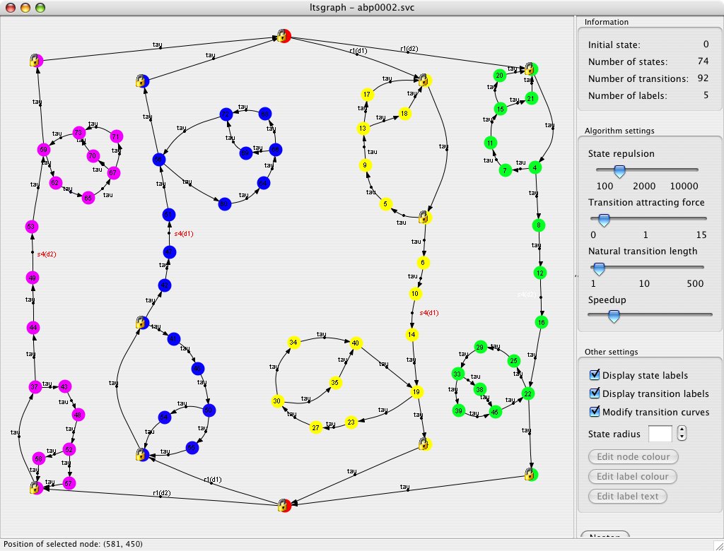
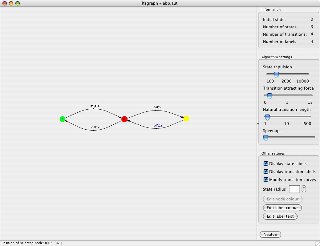
If hiding is applied, the process behaviour can be reduced modulo branching
bisimulation. Under the assumption that empty multi-actions (i.e. tau
actions) cannot be observed, the behaviour of a transition system becomes much
smaller. For example for the alternating bit protocol the picture below on the
left depicts the behaviour before branching bisimulation reduction is applied,
and the picture on the right depicts the equivalent reduced behaviour.
|
|
Time
Using the @ operator it can be expressed at which time an action can take
place. In the process a@1 . b@3 . c@8 we see three actions taking place at
time instances 1, 3 and 8. The time labels are positive Real numbers,
meaning that we use absolute, dense time. If actions do not carry an explicit
time, they can take place at any time instance.
Actually, the time operator applies to processes in general. The process p@t
represents the process where the first action of p must take place at time
t. If timing constraints conflict, e.g. in a@3@5, the process time
deadlocks meaning that the time cannot proceed from a certain moment onwards.
Although this cannot happen in reality, time deadlocks are a strong tool to
investigate that all time constraints in a behavioural specification are
consistent. A time deadlock is written as delta@t. More concretely, the
process above is equal to delta@3.
Although labelling an action with time is rather straightforward, it is a very versatile tool in the context of conditions and sum operators. For instance, a clock that ticks every second is specified by
Clock(t: Real) = tick@(t + 1) . Clock(t + 1);
We can make a drifting clock as follows (where e is some small constant):
Clock(t: Real) =
  sum u: Real . (1 - e <= u && u <= 1 + e) -> tick@(t + u) . Clock(t + u);
A timeout can be specified in much the same way. If the action water must
follow within five time units after the action fire, then this can be
specified by the following expression:
...
sum t: Real . fire@t . sum u: Real. (u <= 5) -> water@(t + u)
...
Processes with time can be linearised and using the lpsuntime tool time annotation can be removed (preserving the time induced orders on processes). Also checking timed modal formulas is possible. Due to the fact that time ranges over real numbers, it is generally not possible to simulate processes that use explicit time, or to generate their state space.